ICT Networks in Building Services

Introduction

ICT networks in building services consist of the structured cabling and associated equipment used to transmit data within and between building systems. These networks support a wide range of services, including IT systems, telephony, building management systems (BMS), instrumentation, and security systems such as CCTV and access control.

From an electrical engineering perspective, ICT networks form part of the extra-low voltage (ELV) infrastructure. Their design must be coordinated with power distribution, cable containment, earthing arrangements, and overall equipment layout within the building.

The design of an ICT network is influenced by several factors, including building layout, the number and distribution of data points, redundancy requirements, segregation from LV systems, electromagnetic interference (EMI), and provision for future expansion.

Consideration must also be given to relevant standards for structured cabling, the location of equipment such as data cabinets and communications rooms, and the environmental conditions in which the system will operate.

This report covers the following:

• The role of ICT networks within building services
• Key design factors influencing their implementation
• Typical equipment and infrastructure used

OSI Model – Purpose and Associated Equipment

The OSI model is a conceptual framework used to describe how data moves through a network. It breaks communication into seven layers, each with a specific role. In practice, not every layer maps cleanly to a physical device, but the model is useful for understanding how different parts of a network interact.

At the lowest level is the Physical Layer (Layer 1). This is concerned with the transmission of raw signals. It defines how bits are carried over a medium, whether copper or fibre. In building services, this corresponds to the physical infrastructure: cables, connectors, patch panels, and fibre links. Devices such as patch panels and cabling systems operate at this level.

Component	Purpose
Copper cables (e.g. Cat6A)	Transmit electrical signals between devices within the network
Fibre optic cables	Transmit data as light signals over long distances and at high bandwidth
Data outlets (RJ45 sockets)	Provide the physical interface for end devices to connect to the network
Patch panels	Terminate and organise fixed cabling, enabling flexible connections
Patch leads	Connect patch panels to switches or devices
Connectors (RJ45, LC, SC)	Provide physical connection points between cables and equipment
Cable containment (tray, basket, trunking)	Support and route cables throughout the building
Racks / cabinets	House and organise network equipment and cabling
SFP/SFP+ modules	Interface fibre cables with network devices (convert electrical ↔︎ optical)
Media converters	Convert signals between copper and fibre where required

Data Link Layer (Layer 2) – Connects devices

The Data Link Layer is responsible for moving data between devices on the same local network.

Every device on a network (such as a laptop, camera, or control panel) has a unique physical address, known as a MAC address. The Data Link Layer uses these addresses to make sure data is sent to the correct device within that local network.

This is the layer at which network switches operate. A switch receives data, checks the destination address, and forwards it only to the correct port, rather than sending it to every device. This makes communication efficient and avoids unnecessary traffic.

In simple terms, the Data Link Layer controls how devices on the same network talk to each other and ensures that data reaches the correct destination within that network.

Component	Purpose
Network switch	Connects data circuits and directs traffic between them. A Layer 2 switch moves data within the same network.

Network Layer (Layer 3) – Connects networks

The Network Layer is responsible for moving data between different networks.

Up to the Data Link Layer, communication only works within the same local network. The Network Layer takes over when data needs to travel further, for example from one part of a building to another, or from your building to the internet.

At this level, devices are identified using logical addresses, known as IP addresses. Unlike MAC addresses (which are fixed to a device), IP addresses are used to organise devices into networks and allow communication between them.

When data is sent, the Network Layer decides where it needs to go and how to get there. It does this by selecting a path through the network, passing the data from one device to another until it reaches its destination. This process is known as routing.

Routers and Layer 3 switches operate at this layer. These devices examine the destination IP address and determine the best path for the data to follow. For example, a router may send traffic from a local building network out to an external network, while a Layer 3 switch may direct traffic between different internal networks within the same building.

In simple terms, the Network Layer acts like a navigation system. It looks at where the data needs to go and chooses the route to get it there, even if it has to pass through multiple networks along the way.

Component	Purpose
Router	Directs data between different networks (e.g. building ↔︎ internet)
Layer 3 Switch	Routes traffic between internal networks (subnets) within a building A Layer 3 switch can also move data between different networks.
Firewall	Controls and secures traffic between networks

The Transport Layer (Layer 4) – Software Logic is responsible for end-to-end communication between devices. It ensures that data is delivered reliably, in the correct order, and without loss where required.

Protocols such as TCP and UDP operate at this layer. This layer is typically implemented in software within devices (i.e. servers, switches, PCs) rather than being tied to specific hardware.

The Session Layer (Layer 5) manages communication sessions between applications. It establishes, maintains, and terminates connections. While not associated with specific physical equipment, its functions are handled by operating systems and network services.

The Presentation Layer (Layer 6) ensures that data is in a usable format. It handles data encoding, encryption, and compression. For example, converting data into a standard format or encrypting it for secure transmission. Like the session layer, this is implemented within software rather than dedicated hardware.

At the top is the Application Layer (Layer 7), which provides the interface between network services and user applications. This is where protocols such as HTTP, FTP, and SMTP operate. Servers, client applications, and network services interact at this level, although the underlying processing spans multiple layers beneath.

In practical building services design, the lower layers (Physical, Data Link, and Network) are the most relevant, as they relate directly to cabling, switches, and routing infrastructure. The upper layers are largely handled by software systems and applications, but they depend on the correct design and installation of the lower layers to function reliably.

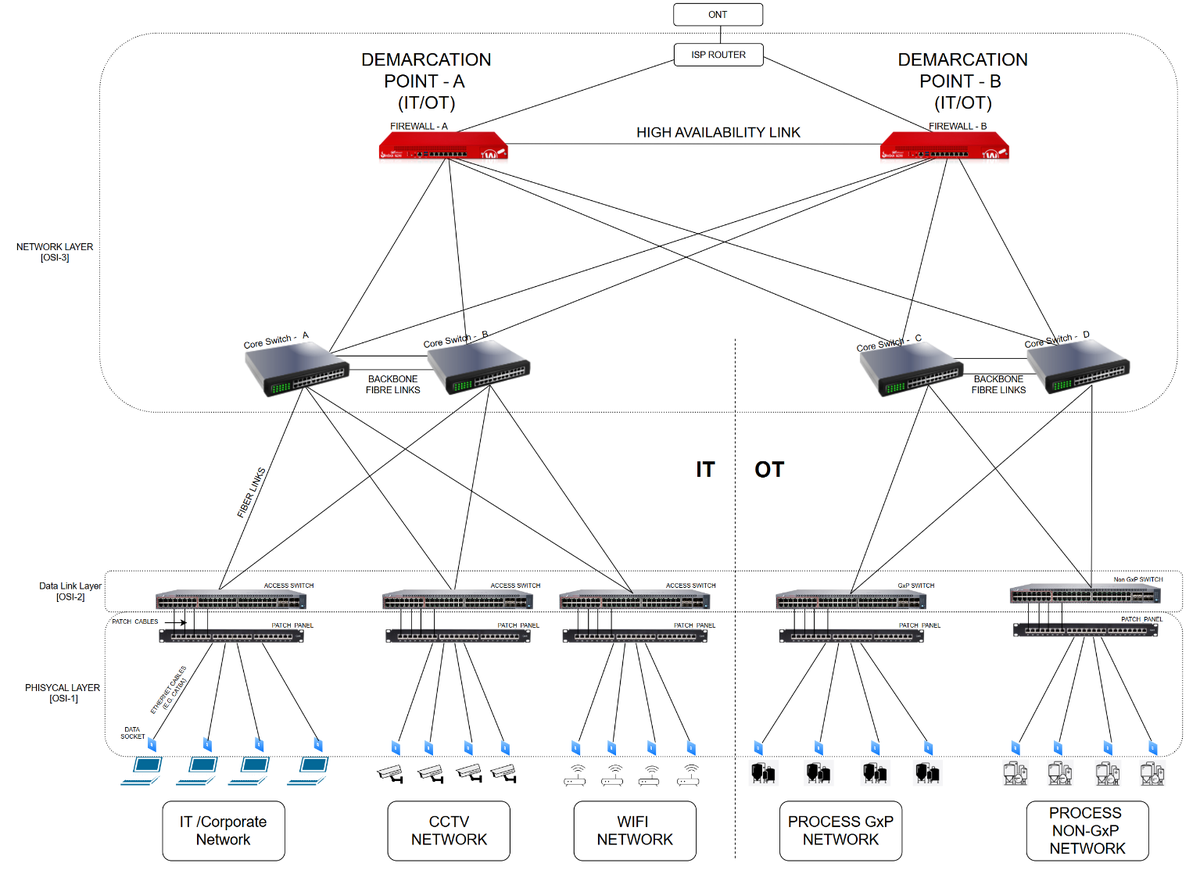
Demarcation Point between Instrumentations and Enterprise Network

In modern facilities, particularly within industrial and pharmaceutical environments, instrumentation and control systems are often required to exchange data with enterprise IT systems. However, these two domains have fundamentally different requirements. Instrumentation networks are designed for reliability, determinism, and process integrity, while enterprise networks prioritise flexibility, accessibility, and user-driven communication. For this reason, a clear demarcation point must be established between them.

An OT (Operational Technology) Network, typically includes:

• BMS (Building Management System)
• PLC / DCS control systems
• Instrumentation (sensors, actuators)
• SCADA systems
• Process equipment

The demarcation point represents the defined boundary at which the instrumentation OT network interfaces with the enterprise (IT) network. At this boundary, communication is controlled, monitored, and, where necessary, restricted. The objective is to allow only the required data to pass between systems, while preventing unintended interactions that could compromise process operation or security.

From a physical and architectural perspective, the demarcation point is typically implemented within the main communications room or control room, using dedicated network equipment. This commonly includes firewalls or managed Layer 3 switches configured to enforce network segmentation. Instrumentation systems are connected to one side of this boundary, while enterprise systems connect to the other. The two networks remain logically and physically separated, even if they share certain infrastructure elements.

A key function of the demarcation point is to control traffic between networks. Instrumentation systems often require predictable and stable communication, and may be sensitive to latency, broadcast traffic, or external interference. Direct integration with enterprise networks can introduce uncontrolled traffic patterns and increase the risk of disruption. By enforcing segregation at the demarcation point, only authorised and necessary communication paths are permitted.

In regulated environments, such as GxP facilities, the demarcation point also supports compliance by clearly defining system boundaries. This enables validation, change control, and security responsibilities to be managed independently for instrumentation and enterprise systems.

In summary, the demarcation point is not simply a connection between two networks, but a controlled interface that ensures secure, reliable, and well-defined communication between fundamentally different system environments.

Network Topologies

A network topology defines the physical and logical arrangement of connections between devices within a network. In the context of building services, the selected topology influences how data is distributed, how faults propagate through the system, and how easily the network can be expanded or maintained.

Star Configuration

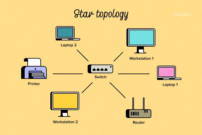
The most widely adopted topology in modern ICT installations is the star configuration. In this arrangement, each device or data outlet is connected via a dedicated cable back to a central switch, typically located within a local communications cabinet. This approach aligns with the principles of structured cabling, where all field cables terminate at patch panels and are then connected to active equipment. The primary advantage of the star topology is that faults are localised; a failure in a single cable or outlet affects only that connection, without impacting the wider network. This makes it particularly suitable for building environments where reliability and ease of fault finding are important.

At a higher level within the network architecture, such as between communication rooms or core equipment, variations of mesh or redundant topologies may be introduced. In these arrangements, multiple paths are provided between switches, allowing data to be rerouted in the event of a link or equipment failure. While more complex, this approach improves resilience and is often used in critical installations or where continuous operation is required.

Other topologies, such as bus and ring configurations, are less commonly used in building ICT networks. Bus topologies, where multiple devices share a single communication path, are largely obsolete due to their lack of fault tolerance and scalability. Ring topologies, in which devices are connected in a closed loop, are still encountered in certain industrial or control system applications, where deterministic communication or built-in redundancy is required.

In practice, most building ICT networks adopt a hybrid approach. A star topology is typically used at the access level to connect end devices, while more resilient configurations are implemented at the backbone or core level to improve overall system reliability. This combination provides a balance between simplicity, performance, and fault tolerance, and reflects the operational requirements of modern building services.

Structured Cabling

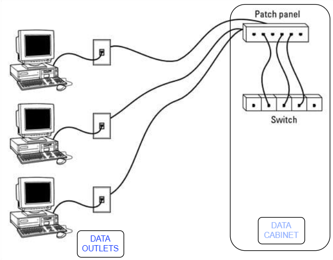
ICT networks are installed using a structured cabling system. This means one common cabling network is installed throughout the building, and different systems are connected to it as required.

The system generally includes:

• Cables from cabinets to outlets
• Backbone cables between cabinets (often fibre)
• Patch panels (panel in a data cabinet where cables connecting data outlets are terminated)
• Data cabinets with network equipment

Type of Cables

Four major types of communications media (cabling) are available for data networking today:

• Unshielded twisted pair (UTP)
• Shielded or screened twisted-pair (STP or ScTP)
• Coaxial
• Fibre Optic (FO)

It is important to distinguish between backbone cables and horizontal cables.

• Backbone cables connect network equipment such as servers, switches, and routers and connect equipment rooms and telecommunications rooms.
• Horizontal cables run from the telecommunications rooms to the wall outlets.

Unshielded Twisted Pair (UTP)

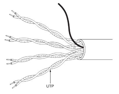
They are the standard medium for Ethernet LANs (Cat5e, Cat6, Cat6A) in offices, data centres, and industrial buildings, supporting up to 10 Gb/s over 100 m depending on category. UTP remains preferred due to low cost, ease of installation, and compliance with ISO/IEC 11801 and TIA-568 structured cabling standards.

Shielded Twisted Pair (STP)

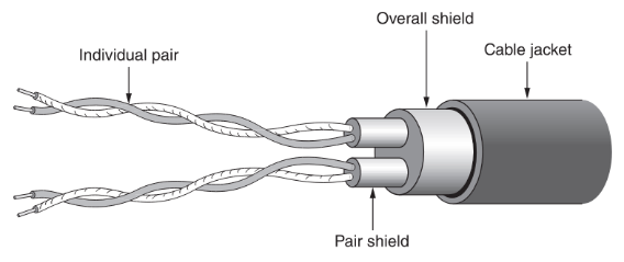
STP (Shielded Twisted Pair) adds an overall shield (foil or braid) and/or individual pair shields to reduce EMI and alien crosstalk. It is used where external noise is high or cable density is extreme (plants with VFDs, data centres, industrial areas).

If bonding is poor, STP can perform worse than UTP due to ground loops or acting as an antenna. STP cable is less susceptible to outside electromagnetic interference (EMI) than UTP cabling because all cable pairs are well shielded.

Constructions of STP in 24 AWG, identical in copper conductor size to UTP cables, are more commonly used today. Simply installing STP cabling does not guarantee you will improve a cable’s immunity to EMI or reduce the emissions from the cable. Several critical conditions must be met to achieve good shield performance:

• The shield must be electrically continuous along the whole link.
• All components in the link must be shielded. No UTP patch cords can be used.
• The shield must fully enclose the pair, and the overall shield must fully enclose the core. Any gap in the shield covering is a source of EMI leakage.
• The shield must be bonded to earth at both ends of the link, and the building earthing system.

Screened Twisted Pair (ScTP)

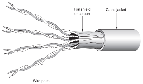
A recognized cable type in the ANSI/TIA-568-C standard is screened twisted-pair (ScTP) cabling, a hybrid of STP and UTP cable.

ScTP cable contains four pairs of unshielded 24 AWG, 100 ohm wire surrounded by a foil shield and a drain wire for bonding purposes. Therefore, ScTP is also sometimes called foil twisted pair (FTP) cable because the foil shield surrounds all four conductors. ScTP cable is essentially STP cabling that does not shield the individual pairs; the shield may also be smaller than some varieties of STP cabling. The foil shield is the reason ScTP is less susceptible to noise. To implement a completely effective ScTP system, the shield continuity must be maintained throughout the entire channel, including patch panels, wall plates, and patch cords.

Like STP cabling, the entire system must be bonded to earth at both ends of each cable run, or the cable will act as a massive antenna, the frequencies of which are inversely proportional to the length of the shield. The net effect is that the noise is out of band.

ScTP is recommended for use in environments that have abnormally high ambient electro-magnetic interference, such as industrial workspaces, hospitals, airports, and government/military communications centres. For example, ScTP is used in fast-food restaurants that use wireless headsets for their drive-through-window workers; some wireless frequencies can interfere with Ethernet over copper.

Bandwidth, Frequency, and Data Rate

One initially confusing aspect about cabling is that cables are rated in hertz rather than bits per second. Network engineers are more concerned with how much data can be pushed through the cable than with the frequency at which that data is traveling.

Frequency is the number of cycles completed per unit of time and is generally expressed in hertz (cycles per second).

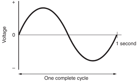
Data cabling is typically rated in kilohertz (kHz) or megahertz (MHz). For a cable rated at 100MHz, the cycle would have to complete 100,000,000 times in a single second! The more cycles per second, the more noise the cable generates and the more susceptible the cable is to signal level loss.

The bandwidth of a cable is the maximum frequency at which data can be effectively transmitted and received. The bit rate is dependent on the network electronics, not the cable, provided the operating frequency of the network is within the cable’s usable bandwidth. Put another way, the cable is just a pipe. Think of the bandwidth as the pipe’s diameter. Network electronics provide the water pressure.

Cable bandwidth is a difficult animal to corral. It is a function of three interrelated, major elements:

• Distance
• Frequency
• Signal-level-to-noise-level ratio (SNR).

Changing any one element alters the maximum bandwidth available. As you increase the frequency, SNR gets worse, and the maximum bandwidth is decreased. As you increase distance, SNR worsens, thereby decreasing the maximum bandwidth. Conversely, reducing frequency or distance increases the maximum bandwidth because SNR improves.

To keep the same maximum bandwidth, increasing the frequency means you must either decrease distance or improve the signal level at the receiver. If you increase the distance, either the frequency must decrease, or, again, the signal level at the receiver must improve. If you improve signal level at the receiving end, you can either increase frequency or leave the frequency alone and increase distance.

Network cabling design is standardised to manage the many variables that affect performance, primarily through IEEE Ethernet specifications and ANSI/TIA-568 structured cabling standards. These standards fix the maximum horizontal cable length at 100 m, including patch leads, due to Ethernet timing constraints, ensuring universal compatibility across current and future LAN technologies.

With distance and frequency fixed, cable design focuses on maximising signal integrity and minimising noise to achieve acceptable signal-to-noise ratio (SNR).

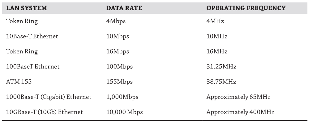
Modern LAN technologies further increase data throughput by encoding multiple bits per hertz, allowing higher data rates without proportionally increasing frequency, though all but the highest-performance systems operate on Category 5 or better cabling.

Category	Typical Data Rates	Typical Max Distance	Typical Use	Key Characteristics
Cat5e	1 Gbps	100 m	Legacy / low-demand systems	Basic performance, largely superseded
Cat6	1 Gbps (10 Gbps up to ~55 m)	100 m	General office networks	Improved performance over Cat5e
Cat6A	10 Gbps	100 m	Modern installations, high-density networks	Higher bandwidth, better noise performance
Cat7*	10 Gbps+	100 m	Specialist applications	Fully screened, not widely used in standard RJ45 systems

Fibre Optic Cable

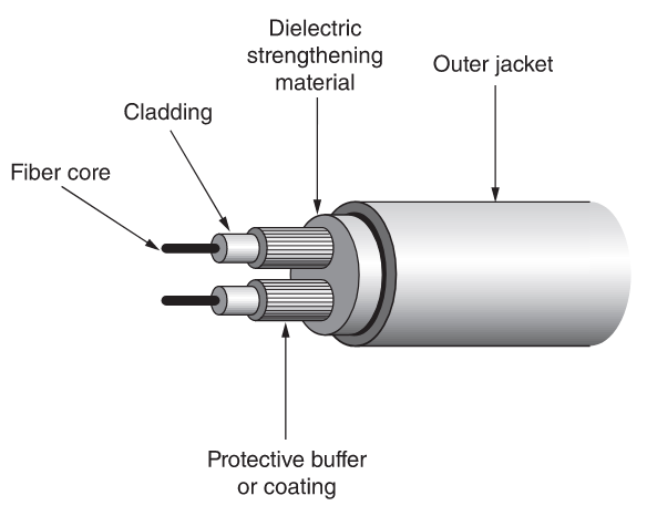
Fibre-optic cable uses a strand of glass or plastic to transmit data signals using light; the data is carried in light pulses. Unlike the transmission techniques used by copper cables, optical fibres are not electrical in nature. Two varieties of fibre-optic cable are commonly used today:

• Single mode
• Multimode

The mode can be thought of as bundles of light rays entering the fibre; these light rays enter at certain angles.

Single-Mode Fibre Optic Cable

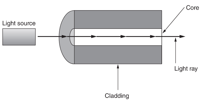
Single-mode fibre-optic cable is most commonly used by telephone companies in data installations as backbone cable interconnecting buildings. Single-mode fibre-optic cable is not used as horizontal cable to connect computers to hubs and is not often used as a cable to interconnect telecommunications rooms to the main equipment room. The light in a single-mode cable travels straight down the fibre and does not bounce off the surrounding cladding as it travels.

Multimode Fibre-Optic Cable

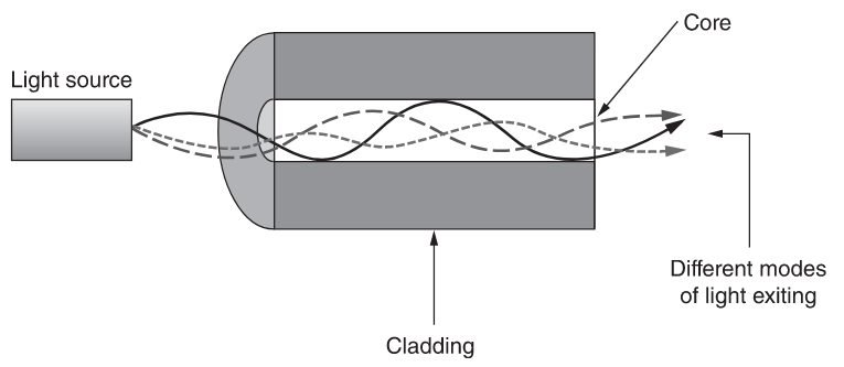
Multimode fibre (MMF) optic cable is usually the fibre-optic cable used with networking applications such as 10Base-FL, 100Base-F, FDDI, ATM, Gigabit Ethernet, 10 Gigabit Ethernet, 40 Gigabit Ethernet, and 100 Gigabit Ethernet that require fibre optics for both horizontal and backbone cable. Multimode cable allows more than one mode (a portion of the light pulse) of light to propagate through the cable.

There are two types of multimode fibre-optic cable:

• step index
• graded index

In step-index multimode fibre, the core has a uniform refractive index with an abrupt boundary to the cladding, causing different propagation modes to travel at significantly different velocities and resulting in high modal dispersion and limited bandwidth/distance performance.

In graded-index multimode fibre, the refractive index gradually decreases from the centre of the core towards the cladding, so higher-order modes travel faster and compensate for longer path lengths, substantially reducing modal dispersion.

As a result, graded-index MMF supports much higher data rates and longer transmission distances and is therefore the standard used in modern installations (OM1–OM5), while step-index MMF is largely obsolete and confined to legacy or very short links.

Graded-index fibre is typically preferred because less light is lost as the signal travels around bends in the cable; therefore, the cable offers much greater bandwidth.

Fibre Type	Typical Distance	Typical Data Rates	Typical Use	Key Characteristics
SMF	Long distance, typically several km	1G, 10G, 25G, 40G, 100G+	Incoming telecoms services, long backbone connections	Very high bandwidth, low attenuation, suited to long-distance transmission
MMF/OM3	Up to ~300 m at 10G	10G, 40G, 100G	High-speed internal building links, MDF to IDF links, internal backbone, data links	Laser-optimised multi-mode fibre
MMF/OM4	Up to ~550 m at 10G	10G, 40G, 100G	Higher performance internal backbone links	Greater distance and bandwidth performance than OM3

What is Dark Fibre

Dark fibre is not a special, new type of fibre cable. When telecommunications companies and private businesses run fibre-optic cable, they never run the exact number of strands of fibre they need. They run two or three times the amount of fibre they require. The spare strands of fibre are often called dark fibre because they are not then in use, that is they don’t have light passing through them.

ICT Network Entry into the Building

Incoming Connection

The ICT network enters the building via a fibre optic cable provided by a telecommunications provider. The cable(s) is routed from the external network (street cabinet or exchange) into the building through underground ducts.

Point of Entry (POE)/Building Entry Point (BEP) and Termination

The fibre enters the building at a defined Point of Entry (POE).

At this location:

• The fibre cable is brought into the building via duct
• The outer sheath is removed
• Individual fibres are terminated (spliced or connectorised)
• Fibres are installed into a fibre termination box or patch panel

This creates a fixed, labelled connection point.

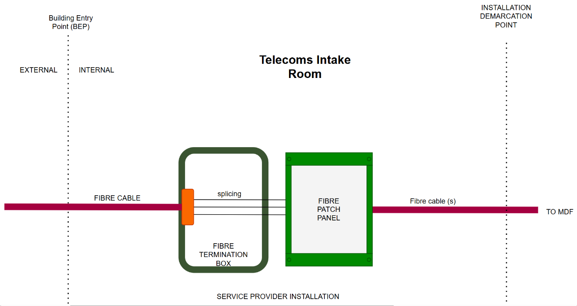
Location of Point of Entry

The POE can be arranged in two ways, depending on project requirements:

Option A – POE within MDF (typical for standard buildings):

• Incoming fibre is routed directly to the MDF
• Termination and active equipment are located in the same room
• Service provider requires controlled access to the MDF

Option B – Separate Intake / Entry Room (for secure or large sites):

• Fibre terminates in a dedicated telecom intake room near the building perimeter with dedicated access for the service provider
• Service provider equipment is installed in this room
• An internal fibre link is run from the intake room to the MDF
• Access to the MDF remains restricted

Main Distribution Frame (MDF)

The MDF is the main communications room where the building’s internal network is established. It typically contains:

• Core switches
• Access Switches
• Routers
• Firewalls
• Fibre backbone connections to other cabinets (IDFs)

All internal ICT distribution originates from the MDF.

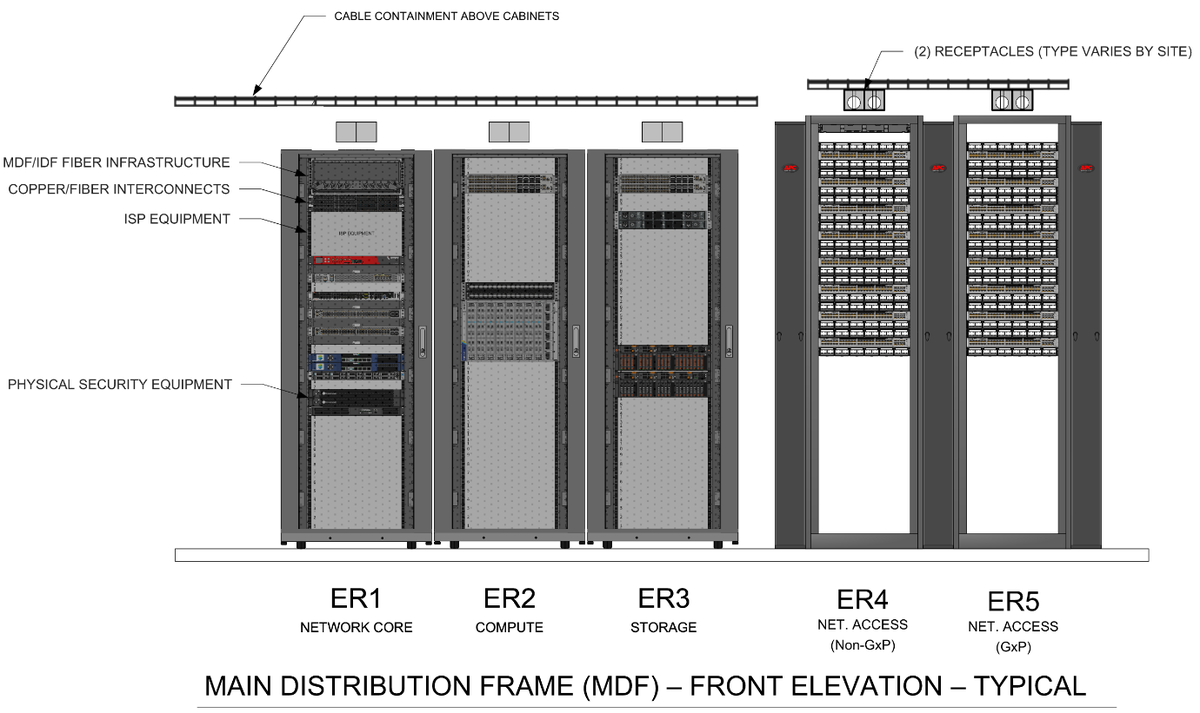
ER1 – Core	ER2 – Compute	ER3 – Storage	ER4 – Non GxP	ER5 – GxP
• Core switching equipment • Main network backbone node Connects: ISP / incoming services, all access switches (ER4/ER5), backbone links (other IDFs) This is the central traffic hub	• Servers / virtualisation hosts • Runs applications, services, VMs • Connected to core for data access This is where processing happens	• Data storage systems (SAN/NAS) • Holds application data, backups, databases • High-speed links to compute and core This is where data lives	• Access switches serving non-regulated systems Typical loads: utilities monitoring, office IT, Wi-Fi, admin systems, BMS (non-critical) Lower compliance requirements	• Access switches for regulated systems Supports: BMS (critical), environmental monitoring, production systems (EMS, DCS, PCS) Requires: segregation, controlled access, validation, restricted access Higher compliance requirements

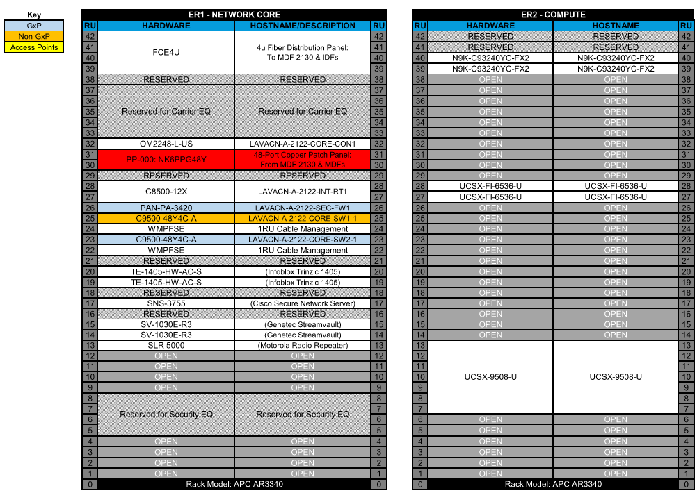
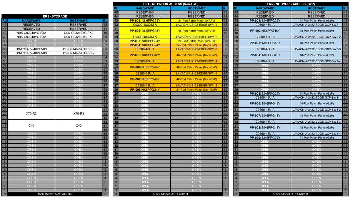
Actual example of data racks and equipment models/type (MDF Room). GxP – GMP lab equipment; Non-GxP – general equipment (BMS, CCTV, access control, IT network except Wi-Fi); Access Points – wireless access points:

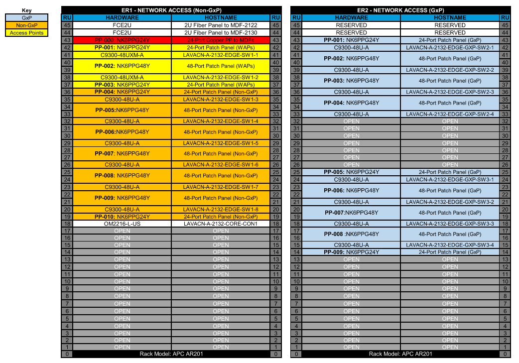
Actual example of data racks and equipment models/type (IDF Room):

Intermediate Distribution Frame (IDF)

The IDF is a local communications room or cabinet serving a defined area or floor of the building. It typically contains:

• Access switches
• Patch panels for horizontal cabling
• Distribution Switches
• Fibre or copper uplinks back to the MDF

The IDF distributes ICT services from the MDF to end devices within its coverage area.

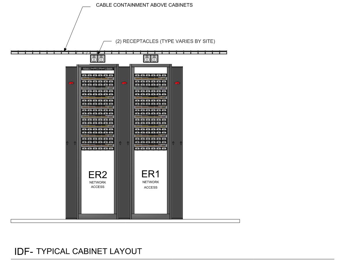
ER1 – Access + Non GxP	ER2 – Access GxP
• Access switches serving non-regulated systems Typical loads: office IT, Wi-Fi, admin systems, BMS (non-critical), process – non-critical Lower compliance requirements	• Access switches for regulated systems Supports: BMS (critical), environmental monitoring, production systems (EMS, DCS, PCS) Requires: segregation, controlled access, validation Higher compliance requirements

Design Considerations

The electrical designer must coordinate:

• Duct routes from site boundary to POE
• Location of POE and MDF (distance, accessibility, security)
• Containment for fibre and data cabling
• Segregation from LV power cables
• Power supplies for active ICT equipment (including UPS where required)
• Earthing and bonding of cabinets and containment
• Fire stopping at all cable entry points
• Security requirements (provider access vs restricted areas)
• Future capacity for additional services

Determining Number of Data Cabinets Needed for a Building

Each device comes in a form factor named “U” which is the device unit height:

• 1U device → 44.45 mm tall

The physical height (U factor) depends on the internal components (i.e. cooling, power, port density). Therefore, a data cabinet may be described as:

• 42U (standard/most common)
• 12U–18U wall mounted / very small setups

A 42U cabinet is defined by height: 42U = 42 × 44.45 mm = 1867 mm usable height.

Typical external dimensions [42U cabinet]: height ~2000 mm (2.0 m); width 600 mm or 800 mm; depth 800 mm, 1000 mm, or 1200 mm.

A typical data cabinet comprises a number of devices:

• Servers to run applications and processing data – 1U/2U
• Switches to connect devices and move network traffic – 1U/2U
• Patch panels for field cables – 1U/2U
• Storage to store data and for backups – 2U/4U
• UPS units to provide backup power to the cabinet, when a UPS-backed supply is not available – 2U/6U
• Security devices (firewall/VPN, traffic filtering) – 1U
• NVR (Network Video Recorder – if CCTV required) – 1U/2U
• Video Management Service (if not included in NVR) – 1U/2U video server
• Cable management – 4U
• Spare capacity – 25%

Working Example – Determining Number of Cabinets Required for a Building

Step 1. Determine the number of data points in the building

• Assuming a single communication room required (MDF)
• Assuming 1000 data points
• Non-GxP points only
• 25% future spare
• 20% space for cable management (8U)
• Patch panel size = 1U = 24 ports; 2U = 48 ports
• Switch size = 1U / 48 ports

Number of ports required (with 25% future spare) = 1250

Number of points ÷ ports per patch panel = 1250 ÷ 24 = 52.08 ≈ 53U

Step 2. Determine size of data cabinet accommodating data points

Data Cabinet 01: UPS: 6U; space for cable management: 8U. Actual available space = 42U – 14U = 28U.

a) Switch type/size	1 x switch (48 ports) = 1U
b) Patch panel type/size	1 x patch panel (48 ports) = 2U

As per a & b above, one 3U configuration = 48 ports

28U ÷ 3U = 9.33 ≈ 9 configurations per data cabinet

Total number of points per cabinet: 9 configs × 48 ports = 432 data points

Number of cabinets to serve field data points: 1250 ÷ 432 = 2.89 ≈ 3 cabinets

Total number of cabinets for the MDF:

Data Cabinet 1 – Core Switching	Data Cabinet 2 – Access	Data Cabinet 3 – Access	Data Cabinet 4 – Access
Core switch, compute server, security server, data storage, UPS	Access switches serving non-regulated systems: office IT, Wi-Fi, admin systems, BMS (non-critical)	Access switches serving non-regulated systems: office IT, Wi-Fi, admin systems, BMS (non-critical)	Access switches serving non-regulated systems: office IT, Wi-Fi, admin systems, BMS (non-critical)
42U — 2m (H) x 0.8m (W) x 1m (D)	42U — 2m (H) x 0.8m (W) x 1m (D)	42U — 2m (H) x 0.8m (W) x 1m (D)	42U — 2m (H) x 0.8m (W) x 1m (D)

Determining Number of ICT Communication Rooms (MDFs/IDFs)

This is typically based on the following factors:

1. Horizontal cabling distance

• Maximum allowed length for a CAT6 cable to operate reliably is typically 100 m (90 m cable run + 10 m patch lead). Beyond that, signal attenuation increases (weaker signal), noise/crosstalk impact increases, bit errors increase, and the link may drop to lower speed or fail completely. So each cabinet can only serve outlets within a 90 m radius/path length.

2. Number of data points in each area

• Even if distance is fine, one room may not have enough rack space or switch capacity. High-density areas may need their own local cabinet.

3. Building layout

• Multiple floors, fire compartments, physical barriers (these often force additional ICT rooms)

4. Segregation requirements

• GxP / non-GxP, security systems, operational separation (these may require separate cabinets or rooms)

5. Resilience / operational requirements

• Critical areas may need local IDFs; redundant routing may influence room locations

6. Available space

• Requirements for ICT rooms include power, cooling/ventilation, access control, and containment routes

Earthing and Bonding

In ICT installations, the use of a dedicated earth connection for ICT equipment is driven by the need for a controlled and predictable bonding arrangement, rather than relying on distributed or daisy-chained earth connections between equipment.

In a daisy-chain arrangement, equipment racks and containment are bonded sequentially, with each item relying on the previous one to provide a path to earth. This creates a shared earthing path with cumulative impedance. As a result, voltage differences can develop between items of equipment, particularly under fault conditions or in the presence of electromagnetic noise. These differences can drive circulating currents through equipment frames and cable screens, leading to electromagnetic interference and degraded system performance.

In addition, the integrity of the earthing system becomes dependent on each intermediate connection, making it more vulnerable to poor workmanship and difficult to verify.

A dedicated earth bar eliminates these issues by establishing a radial (star) bonding arrangement. All ICT equipment, including racks, patch panels, and metallic containment, is bonded individually to a single local earth bar, which is in turn connected to the building’s Main Earthing Terminal (MET). This provides each item with a direct, low impedance path to earth, independent of other equipment.

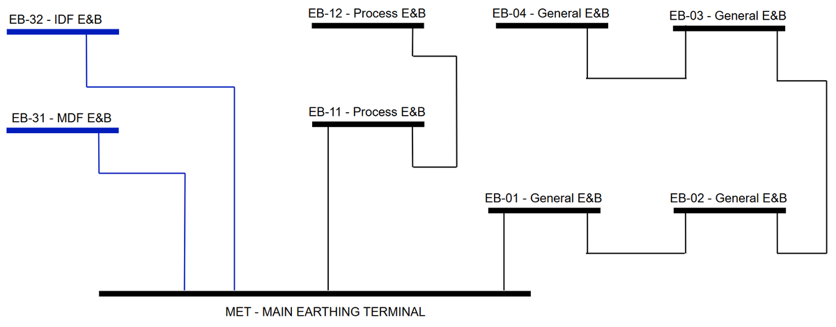
By maintaining a common reference point and minimising shared impedance, the dedicated earth bar reduces the risk of potential differences and circulating currents. This improves electromagnetic compatibility, supports the correct operation of screened cabling systems, and ensures more reliable performance of network equipment.

In addition, a centralised bonding point provides a clear and accessible location for inspection and testing, allowing the earthing arrangement to be verified more easily against relevant standards.

Overall, the dedicated earth bar enables a controlled, robust, and maintainable earthing strategy, which is essential for the reliable operation of modern ICT systems.

Earthing of ICT cabinets:

• Rack / cabinet frame → bond to earth
• Metal containment (tray, ladder, trunking) → bond
• Patch panels (metal) → bonded via rack
• Active equipment (switches, servers) → earthed via PSU
• Cable screens (if screened cables used): ICT structured cabling → screened cables terminated both ends; instrumentation/control → screen earthed at one end only (typical practice)

Structured cabling (Cat6A, Ethernet)	Instrumentation / control cables
Screen (if present) → terminated at both ends	Screen → typically earthed at one end only
Earthing via: patch panel → rack → MET	Usually at: control panel / DCS side
Designed for high-frequency differential signals	Designed for low-level analogue signals
Reason: needs full shielding effectiveness; standards require continuity	Reason: sensitive to noise from circulating currents; one-end earthing avoids loop currents

Instrumentation Cabling

Instrumentation cabling is used to transmit control and monitoring signals between field devices and control systems such as PLCs, DCS, or SCADA. These signals may be analogue (e.g. 4–20 mA), digital, or low-voltage control signals, and are typically of much lower magnitude than power circuits. As a result, instrumentation cables are more sensitive to electrical noise and require careful selection and installation to ensure reliable operation.

Instrumentation cables are generally constructed as twisted pairs or multi-core cables, often incorporating individual pair screening and/or overall shielding. The purpose of this screening is to protect low-level signals from electromagnetic interference, particularly in industrial environments where equipment such as motors, variable speed drives, and switching devices can introduce significant electrical noise.

A key aspect of instrumentation cabling design is the treatment of cable screens. Unlike data cabling systems, where screens are typically terminated at both ends, instrumentation cable screens are generally earthed at one end only, usually at the control panel or system end. This approach minimises the risk of circulating earth currents, which can introduce noise into sensitive analogue signals.

Routing and containment of instrumentation cables must be carefully coordinated to avoid sources of interference. Segregation from power cables is essential, particularly from high-current circuits and those supplying non-linear loads. Where parallel routing is unavoidable, adequate separation distances should be maintained, and crossings should be made at right angles.

Cable selection must also consider the installation environment. External or industrial areas may require armoured cables for mechanical protection, while internal installations may use unarmoured cables within suitable containment systems. In all cases, bending radius, support, and termination practices must be controlled to prevent damage to the cable and maintain signal integrity.

In critical applications, particularly within regulated environments such as pharmaceutical facilities, instrumentation cabling may be associated with GxP systems. In such cases, additional requirements may apply, including segregation, redundancy, and documentation to support system validation.

In summary, instrumentation cabling requires a controlled and disciplined approach to selection, routing, and termination, with particular emphasis on noise mitigation and earthing strategy to ensure accurate and reliable signal transmission.

Cable Containment for ICT Systems

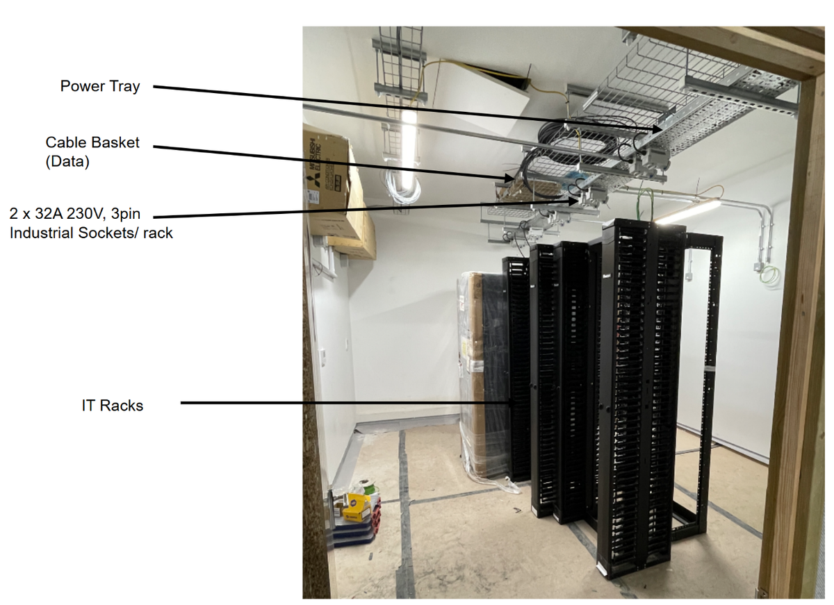
Cable containment provides the physical routing and support for ICT cabling throughout a building and forms an integral part of the overall network infrastructure. In structured cabling systems, containment must be designed not only to carry cables, but also to preserve their performance, allow safe installation, and accommodate future expansion.

Typical containment systems include cable basket, trunking and conduits. Cable baskets are commonly used for main horizontal and vertical distribution routes due to their accessibility, ease of installation, and ability to support large volumes of cabling. Trunking and conduit are generally used in areas requiring increased mechanical protection or where cables are exposed within occupied spaces.

Unlike power systems, the performance of data cabling can be affected by installation conditions. Excessive bending, compression, or overfilling of containment can degrade signal quality, particularly for high-performance cables such as Cat6A. Containment should therefore be sized to avoid overcrowding, allow adequate bend radii to be maintained, and provide sufficient spare capacity for future modifications. As a general principle, containment should not be fully utilised at installation stage.

Segregation from LV power cables is an important consideration in containment design. Copper data cables are susceptible to electromagnetic interference, particularly when installed in parallel with power circuits carrying higher currents or supplying non-linear loads. To mitigate this, data and power cables should be routed on separate containment systems where practicable. Where parallel runs are unavoidable, appropriate separation distances should be maintained, increasing with the magnitude of the adjacent power circuits. In constrained situations, the use of screened data cables and metallic containment can help reduce interference. Where crossings are required, they should be arranged at right angles and over the shortest possible distance.

Fibre optic cables are immune to electromagnetic interference and are not subject to the same performance-related segregation requirements. However, they should still be routed separately from power cables where possible to maintain clear installation practices and reduce the risk of mechanical damage.

Containment routes must be coordinated with the building layout, including risers, ceiling voids, and plant areas, to ensure continuous and accessible pathways between communication rooms and end devices. Particular attention should be given to routing through fire-rated elements, where all penetrations must be appropriately sealed to maintain the fire integrity of the building.

Metallic containment systems should be bonded to the building earthing system to ensure equipotential conditions and support overall electromagnetic compatibility. This is particularly important where screened cabling systems are employed.

In summary, cable containment is not simply a means of supporting cables, but a critical component of the ICT infrastructure that directly influences system performance, maintainability, and long-term adaptability.

Collapsed Core vs 3–Tier Architecture

When designing an ICT network for a building, the way switches are arranged has a direct impact on cost, complexity, and performance. Two common approaches are used:

• The three-tier architecture
• The collapsed core architecture

In a three-tier architecture, the network is divided into three levels. The access layer is where end devices connect, typically through switches located in local communications rooms (IDFs). These access switches connect to a distribution layer, which collects connections from multiple access switches and manages traffic between them. Above this, the core layer forms the backbone of the network, providing high-speed connectivity between different parts of the system. Data travelling across the network passes through each of these layers in sequence. This structure is commonly used in large sites, such as campuses or multi-building developments, where the number of switches and the distances involved require a more scalable and organised approach.

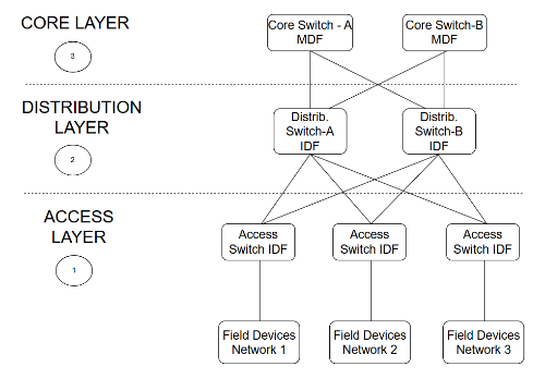
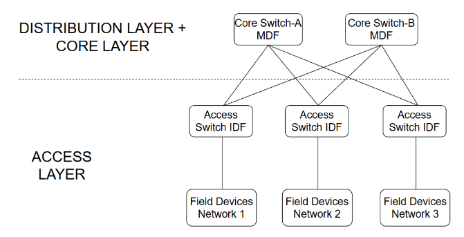
In a collapsed core architecture, the distribution and core layers are combined into a single layer. Access switches connect directly to a central pair of core switches, usually located in the main communications room (MDF). These core switches perform both aggregation and routing functions, meaning they collect connections from access switches and manage communication between different networks. This removes the need for a separate distribution layer, resulting in a simpler network with fewer devices and fewer connections.

For most building services applications, a collapsed core architecture is more appropriate. Buildings typically do not require the level of scale provided by a three-tier design, and introducing additional layers would add unnecessary complexity. A collapsed core reduces the amount of equipment required, simplifies installation, and makes the system easier to understand and maintain. Resilience is still achieved by using two core switches, ensuring that the network continues to operate in the event of a single failure.

In summary, a three-tier architecture separates network functions across multiple layers to support large and complex installations, while a collapsed core architecture combines these functions into a single layer, providing a simpler and more efficient solution for typical building networks.